Loop-soup simulations
Numerical experiments with random-walk loop soups: from planar loop configurations and split-merge dynamics to intersection clusters and small-loop sprinkling in three dimensions.
Download all Python codeSource files and setup
01Planar loop soups
Random walks on a square lattice generate a soup of loops through a Wilson-type construction with a wired boundary. These saved carpet pictures are labelled $N=1000$.


The disk carpet is conformally mapped from the square image. The circular views below instead clip square-lattice paths to a disk; they are not separate disk-domain samples.
02Diameter cutoffs
Retain only loops whose spatial size is at least $\varepsilon$. In the 2D code, size is the maximum coordinate span divided by $N$. Decreasing the cutoff reveals progressively smaller loops.


Circular view at $\varepsilon=0.01$
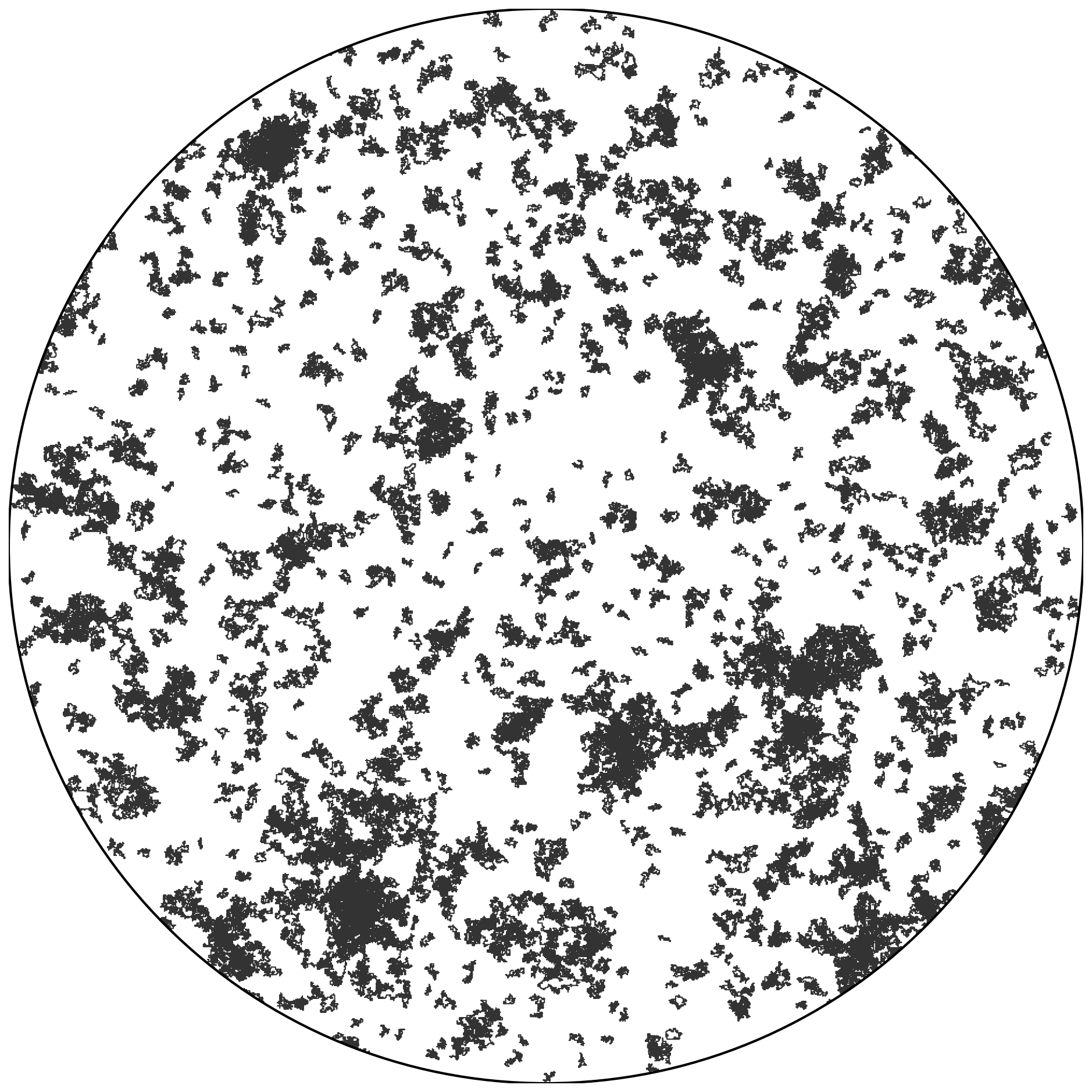
Square cutoff PythonDisk cutoff PythonSquare comparison PythonDisk comparison Python
03Split-merge rewiring
The chain $M^\varepsilon$ splits a loop at a self-intersection or merges two loops at a shared lattice site. Both children of a split must satisfy the diameter cutoff. The animations follow the resulting loop configurations.
Open video
Open video
Open video
Open video
Square PythonDisk PythonSquare comparison PythonDisk comparison Python
04Distance during rewiring
For a fixed observation point $z$, measure the distance to the nearest vertex of each loop, then take the largest of those distances:
$D(t)=\max_{L\in\mathcal{L}_t}\min_{p\in L}\left\|p/(N-1)-z\right\|_2.$
This tracks an observable of the individual loops as the rewiring chain evolves.
Open video
Open video
Open video
Square PythonDisk PythonComparison PythonDesktop interactive Python
05Starting from one loop
Start the same rewiring chain from a single large loop and follow its splitting and merging descendants. The current source selects the largest loop among those retained by the initial diameter filter.
Open video
06Loop soups in three dimensions
The construction extends to a wired $N\times N\times N$ cube. Saved runs use $N=30,50,100,200$ and $c=0.5$. The $N=200$ sample contains 492,614 loops; its viewer displays a filtered subset of 2,905.
N = 200: three-dimensional loop soup
- $N=30$ sample
- $N=50$ sample
- $N=100$ sample
- $N=50$: retained large loops (122 displayed)
3D sampler PythonLarge-loop sampler PythonPlotly viewer PythonCanvas viewer Python
07Intersection clusters
Loops belong to the same cluster when a chain of shared lattice vertices connects them. These $N=200$ views use loops of at least eight steps. One view isolates two clusters; the other identifies a closest pair, separated by one lattice unit.
Two intersection clusters
Closest pair of clusters
08Sprinkling and gluing
Select two clusters formed by loops above a cutoff $L$, then add independent smaller loops in decreasing order of size. The experiment records whether these loops connect the selected clusters and the cutoff at which the first connection appears.
| Run | Dust c | Cutoff window | Outcome |
|---|---|---|---|
| N = 80 | 0.5 | Diameter: 2 ≤ d < 8 | No connection |
| N = 100 | 0.5 | Diameter: 1 ≤ d < 8 | No connection |
| N = 100 | 1.0 | Diameter: 1 ≤ d < 8 | One-loop bridge at d ≈ 7.07 |
| N = 200 | 1.0 | Diameter: 1 ≤ d < 8 | One-loop bridge at d ≈ 7.07 |
| N = 80, local cube | 1.0 | Time length: 2 ≤ ℓ < 8 | One-loop bridge at ℓ = 2 |
Spatial sizes here are bounding-box diagonal lengths in lattice units. The local-cube run uses time length instead. These are individual sample outcomes, not estimates of connection probabilities.
N = 200: a bridge formed by independent dust
N = 80: sprinkling in a local cube
Additional archived runs
Earlier exports of the rewiring and distance experiments, including longer runs and alternative cutoff comparisons. Original filenames identify each recording; complete parameter records were not saved for these variants.
12 additional recordings and figures
- loopsoup-distance copy.gif (50.5 s)
- loopsoup-distance-square.gif (50.5 s)
- loopsoup-distance.gif (25.5 s)
- loopsoup-rewiring copy.gif (41.0 s)
- loopsoup-rewiring-compare copy 2.gif (100.5 s)
- loopsoup-rewiring-compare copy.gif (20.5 s)
- loopsoup-rewiring-compare.gif (5.25 s)
- loopsoup-rewiring.gif (25.25 s)
- loopsoup-rewiring0.001.gif (5.25 s)
- square/loopsoup-distance-square copy.gif (250.5 s)
- square/loopsoup-epsilon-compare-square.png
- square/loopsoup-rewiring-square.gif (41.0 s)

Code and reproduction
Download the complete Python source bundle (24 scripts), or browse the source on GitHub.
The bundle includes the generators, analysis scripts, exporters, and local Streamlit and Flask apps. Export paths are portable; the stochastic logic and parameter defaults are preserved.
python3 -m venv .venv
source .venv/bin/activate
python -m pip install -r requirements.txt

python rwls3d/RWLS_3D.py --N 20 --c 0.5 --seed 11
python rwls3d/app.py --host 127.0.0.1 --port 5055
Full setup and run instructions · Python requirements
For 2D scripts, parameters are constants in each file; start with a small grid. Current source defaults need not match archived runs. In this implementation, $c$ enters a loop-label probability: values above one in some legacy 2D controls saturate. The 3D command-line sampler accepts $0\leq c\leq1$.
All source files
Square-lattice experiments
- RWLS.py
- RWLS_cutoff.py
- RWLS_distance.py
- RWLS_distance_compare.py
- RWLS_distance_interactive.py
- RWLS_epsilon_compare.py
- RWLS_rewiring.py
- RWLS_rewiring_compare.py
- RWLS_single_loop.py
- app.py
Circular visualizations
- RWLS.py
- RWLS_cutoff.py
- RWLS_distance.py
- RWLS_epsilon_compare.py
- RWLS_rewiring.py
- RWLS_rewiring_compare.py